What is Opportunity Cost

Scarcity of resources is one of the more basic concepts of economics. Scarcity necessitates trade-offs, and trade-offs result in an opportunity cost. While the cost of a good or service often is thought of in monetary terms, the opportunity cost of a decision is based on what must be given up (the next best alternative) as a result of the decision. Any decision that involves a choice between two or more options has an opportunity cost.

Opportunity cost contrasts to accounting cost in that accounting costs do not consider forgone opportunities. Consider the case of an MBA student who pays $30,000 per year in tuition and fees at a private university. For a two-year MBA program, the cost of tuition and fees would be $60,000. This is the monetary cost of the education. However, when making the decision to go back to school, one should consider the opportunity cost, which includes the income that the student would have earned if the alternative decision of remaining in his or her job had been made. If the student had been earning $50,000 per year and was expecting a 10% salary increase in one year, $105,000 in salary would be foregone as a result of the decision to return to school. Adding this amount to the educational expenses results in a cost of $165,000 for the degree.
Opportunity cost is useful when evaluating the cost and benefit of choices. It often is expressed in non-monetary terms. For example, if one has time for only one elective course, taking a course in microeconomics might have the opportunity cost of a course in management. By expressing the cost of one option in terms of the foregone benefits of another, the marginal costs and marginal benefits of the options can be compared.

As another example, if a shipwrecked sailor on a desert island is capable of catching 10 fish or harvesting 5 coconuts in one day, then the opportunity cost of producing one coconut is two fish (10 fish / 5 coconuts). Note that this simple example assumes that the production possibility frontier between fish and coconuts is linear.

Relative Price
Opportunity cost is expressed in relative price, that is, the price of one choice relative to the price of another.

For example, if milk costs $4 per gallon and bread costs $2 per loaf, then the relative price of milk is 2 loaves of bread. If a consumer goes to the grocery store with only $4 and buys a gallon of milk with it, then one can say that the opportunity cost of that gallon of milk was 2 loaves of bread (assuming that bread was the next best alternative).

In many cases, the relative price provides better insight into the real cost of a good than does the monetary price.

Applications of Opportunity Cost
The concept of opportunity cost has a wide range of applications including:

* Consumer choice
* Production possibilities
* Cost of capital
* Time management
* Career choice
* Analysis of comparative advantage

Source: www.netmba.com

MBA Notes-The Production Possibility Frontier

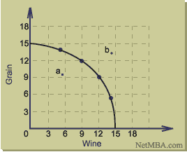
Consider the case of an island economy that produces only two goods: wine and grain. In a given period of time, the islanders may choose to produce only wine, only grain, or a combination of the two according to the following table:

Production Possibility Table

Wine (thousands of bottles)	Grain (thousands of bushels)
0	15
5	14
9	12
12	9
14	5
15	0

The production possibility frontier (PPF) is the curve resulting when the above data is graphed, as shown below:

Production Possibility Frontier

The PPF shows all efficient combinations of output for this island economy when the factors of production are used to their full potential. The economy could choose to operate at less than capacity somewhere inside the curve, for example at point a, but such a combination of goods would be less than what the economy is capable of producing. A combination outside the curve such as point b is not possible since the output level would exceed the capacity of the economy.

The shape of this production possibility frontier illustrates the principle of increasing cost. As more of one product is produced, increasingly larger amounts of the other product must be given up. In this example, some factors of production are suited to producing both wine and grain, but as the production of one of these commodities increases, resources better suited to production of the other must be diverted. Experienced wine producers are not necessarily efficient grain producers, and grain producers are not necessarily efficient wine producers, so the opportunity cost increases as one moves toward either extreme on the curve of production possibilities.

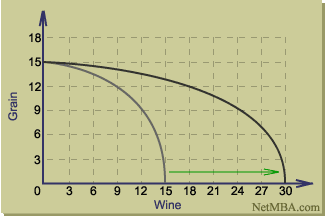
Suppose a new technique was discovered that allowed the wine producers to double their output for a given level of resources. Further suppose that this technique could not be applied to grain production. The impact on the production possibilities is shown in the following diagram:

Shifted Production Possibility Frontier

In the above diagram, the new technique results in wine production that is double its previous level for any level of grain production.

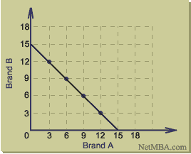
Finally, if the two products are very similar to one another, the production possibility frontier may be shaped more like a straight line. Consider the situation in which only wine is produced. Let's assume that two brands of wine are produced, Brand A and Brand B, and that these two brands use the same grapes and production process, differing only in the name on the label. The same factors of production can produce either product (brand) equally efficiently. The production possibility frontier then would appear as follows:

PPF for Very Similar Products

Note that to increase production of Brand A from 0 to 3000 bottles, the production of Brand B must be decreased by 3000 bottles. This opportunity cost remains the same even at the other extreme, where increasing the production of Brand A from 12,000 to 15,000 bottles still requires that of Brand B to be decreased by 3000 bottles. Because the two products are almost identical in this case and can be produced equally efficiently using the same resources, the opportunity cost of producing one over the other remains constant between the two extremes of production possibilities.

Source: www.netmba.com

MBA Economics Topics-Supply and Demand

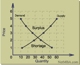
The market price of a good is determined by both the supply and demand for it. In 1890, English economist Alfred Marshall published his work, Principles of Economics, which was one of the earlier writings on how both supply and demand interacted to determine price. Today, the supply-demand model is one of the fundamental concepts of economics. The price level of a good essentially is determined by the point at which quantity supplied equals quantity demanded. To illustrate, consider the following case in which the supply and demand curves are plotted on the same graph.

Supply and Demand

On this graph, there is only one price level at which quantity demanded is in balance with the quantity supplied, and that price is the point at which the supply and demand curves cross.

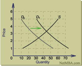
The law of supply and demand predicts that the price level will move toward the point that equalizes quantities supplied and demanded. To understand why this must be the equilibrium point, consider the situation in which the price is higher than the price at which the curves cross. In such a case, the quantity supplied would be greater than the quantity demanded and there would be a surplus of the good on the market. Specifically, from the graph we see that if the unit price is $3 (assuming relative pricing in dollars), the quantities supplied and demanded would be:

Quantity Supplied = 42 units

Quantity Demanded = 26 units

Therefore there would be a surplus of 42 - 26 = 16 units. The sellers then would lower their price in order to sell the surplus.

Suppose the sellers lowered their prices below the equilibrium point. In this case, the quantity demanded would increase beyond what was supplied, and there would be a shortage. If the price is held at $2, the quantity supplied then would be:

Quantity Supplied = 28 units

Quantity Demanded = 38 units

Therefore, there would be a shortage of 38 - 28 = 10 units. The sellers then would increase their prices to earn more money.

The equilibrium point must be the point at which quantity supplied and quantity demanded are in balance, which is where the supply and demand curves cross. From the graph above, one sees that this is at a price of approximately $2.40 and a quantity of 34 units.

To understand how the law of supply and demand functions when there is a shift in demand, consider the case in which there is a shift in demand:

Shift in Demand

In this example, the positive shift in demand results in a new supply-demand equilibrium point that in higher in both quantity and price. For each possible shift in the supply or demand curve, a similar graph can be constructed showing the effect on equilibrium price and quantity. The following table summarizes the results that would occur from shifts in supply, demand, and combinations of the two.

Result of Shifts in Supply and Demand

Demand	Supply	Equilibrium Price	Equilibrium Quantity
+		+	+
-		-	-
	+	-	+
	-	+	-
+	+	?	+
-	-	?	-
+	-	+	?
-	+	-	?

In the above table, "+" represents an increase, "-" represents a decrease, a blank represents no change, and a question mark indicates that the net change cannot be determined without knowing the magnitude of the shift in supply and demand. If these results are not immediately obvious, drawing a graph for each will facilitate the analysis.

Source: www.netmba.com

MBA Economics Topics-The Supply Curve

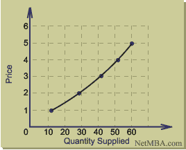
Price usually is a major determinant in the quantity supplied. For a particular good with all other factors held constant, a table can be constructed of price and quantity supplied based on observed data. Such a table is called a supply schedule, as shown in the following example:

Supply Schedule

Price	Quantity Supplied
1	12
2	28
3	42
4	52
5	60

By graphing this data, one obtains the supply curve as shown below:

As with the demand curve, the convention of the supply curve is to display quantity supplied on the x-axis as the independent variable and price on the y-axis as the dependent variable.

The law of supply states that the higher the price, the larger the quantity supplied, all other things constant. The law of supply is demonstrated by the upward slope of the supply curve.

As with the demand curve, the supply curve often is approximated as a straight line to simplify analysis. A straight-line supply function would have the following structure:

Quantity = a + (b x Price)

where a and b are constant for each supply curve.

A change in price results in a change in quantity supplied and represents movement along the supply curve.

Shifts in the Supply Curve

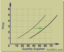
While changes in price result in movement along the supply curve, changes in other relevant factors cause a shift in supply, that is, a shift of the supply curve to the left or right. Such a shift results in a change in quantity supplied for a given price level. If the change causes an increase in the quantity supplied at each price, the supply curve would shift to the right:

Supply Curve Shift

There are several factors that may cause a shift in a good's supply curve. Some supply-shifting factors include:

* Prices of other goods - the supply of one good may decrease if the price of another good increases, causing producers to reallocate resources to produce larger quantities of the more profitable good.
* Number of sellers - more sellers result in more supply, shifting the supply curve to the right.
* Prices of relevant inputs - if the cost of resources used to produce a good increases, sellers will be less inclined to supply the same quantity at a given price, and the supply curve will shift to the left.
* Technology - technological advances that increase production efficiency shift the supply curve to the right.
* Expectations - if sellers expect prices to increase, they may decrease the quantity currently supplied at a given price in order to be able to supply more when the price increases, resulting in a supply curve shift to the left.

Source: www.netmba.com

MBA Economics Topics-Price Elasticity of Demand

An important aspect of a product's demand curve is how much the quantity demanded changes when the price changes. The economic measure of this response is the price elasticity of demand.

Price elasticity of demand is calculated by dividing the proportionate change in quantity demanded by the proportionate change in price. Proportionate (or percentage) changes are used so that the elasticity is a unit-less value and does not depend on the types of measures used (e.g. kilograms, pounds, etc).

As an example, if a 2% increase in price resulted in a 1% decrease in quantity demanded, the price elasticity of demand would be equal to approximately 0.5. It is not exactly 0.5 because of the specific definition for elasticity uses the average of the initial and final values when calculating percentage change. When the elasticity is calculated over a certain arc or section of the demand curve, it is referred to as the arc elasticity and is defined as the magnitude (absolute value) of the following:

Q2 - Q1
--------------------

( Q1 + Q2 ) / 2
--------------------
P2 - P1
--------------------
( P1 + P2 ) / 2

where

Q1 = Initial quantity
Q2 = Final quantity
P1 = Initial price
P2 = Final price

The average values for quantity and price are used so that the elasticity will be the same whether calculated going from lower price to higher price or from higher price to lower price. For example, going from $8 to $10 is a 25% increase in price, but going from $10 to $8 is only a 20% decrease in price. This asymmetry is eliminated by using the average price as the basis for the percentage change in both cases.

For slightly easier calculations, the formula for arc elasticity can be rewritten as:

( Q2 - Q1 ) ( P2 + P1 )
----------------------
( Q2 + Q1 ) ( P2 - P1 )

To better understand the price elasticity of demand, it is worthwhile to consider different ranges of values.

Elasticity > 1

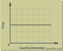
In this case, the change in quantity demanded is proportionately larger than the change in price. This means that an increase in price would result in a decrease in revenue, and a decrease in price would result in an increase in revenue. In the extreme case of near infinite elasticity, the demand curve would be nearly horizontal, meaning than the quantity demanded is extremely sensitive to changes in price. The case of infinite elasticity is described as being perfectly elastic and is illustrated below:

Perfectly Elastic Demand Curve

Elasticity <>
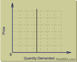
Perfectly Inelastic Demand Curve

From this demand curve, it is easy to visualize how even a very large change in price would have no impact on quantity demanded.

Elasticity = 1

This case is referred to as unitary elasticity. The change in quantity demanded is in the same proportion as the change in price. A change in price in either direction therefore would result in no change in revenue.

Applications of Price Elasticity of Demand
The price elasticity of demand can be applied to a variety of problems in which one wants to know the expected change in quantity demanded or revenue given a contemplated change in price.

For example, a state automobile registration authority considers a price hike in personalized "vanity" license plates. The current annual price is $35 per year, and the registration office is considering increasing the price to $40 per year in an effort to increase revenue. Suppose that the registration office knows that the price elasticity of demand from $35 to $40 is 1.3.

Because the elasticity is greater than one over the price range of interest, we know that an increase in price actually would decrease the revenue collected by the automobile registration authority, so the price hike would be unwise.

Factors Influencing the Price Elasticity of Demand
The price elasticity of demand for a particular demand curve is influenced by the following factors:

* Availability of substitutes: the greater the number of substitute products, the greater the elasticity.
* Degree of necessity or luxury: luxury products tend to have greater elasticity than necessities. Some products that initially have a low degree of necessity are habit forming and can become "necessities" to some consumers.
* Proportion of income required by the item: products requiring a larger portion of the consumer's income tend to have greater elasticity.
* Time period considered: elasticity tends to be greater over the long run because consumers have more time to adjust their behavoir to price changes.
* Permanent or temporary price change: a one-day sale will result in a different response than a permanent price decrease of the same magnitude.
* Price points: decreasing the price from $2.00 to $1.99 may result in greater increase in quantity demanded than decreasing it from $1.99 to $1.98.

Point Elasticity
It sometimes is useful to calculate the price elasticity of demand at a specific point on the demand curve instead of over a range of it. This measure of elasticity is called the point elasticity. Because point elasticity is for an infinitesimally small change in price and quantity, it is defined using differentials, as follows:

dQ

Q

dP

P

and can be written as:

dQ		P
dP		Q

The point elasticity can be approximated by calculating the arc elasticity for a very short arc, for example, a 0.01% change in price.

MBA Economics Topics-The Demand Curve

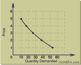
The quantity demanded of a good usually is a strong function of its price. Suppose an experiment is run to determine the quantity demanded of a particular product at different price levels, holding everything else constant. Presenting the data in tabular form would result in a demand schedule, an example of which is shown below.

Demand Schedule

Price	Quantity Demanded
5	10
4	17
3	26
2	38
1	53

he demand curve for this example is obtained by plotting the data:

Demand Curve
By convention, the demand curve displays quantity demanded as the independent variable (the x axis) and price as the dependent variable (the y axis).

The law of demand states that quantity demanded moves in the opposite direction of price (all other things held constant), and this effect is observed in the downward slope of the demand curve.

For basic analysis, the demand curve often is approximated as a straight line. A demand function can be written to describe the demand curve. Demand functions for a straight-line demand curve take the following form:

Quantity = a - (b x Price)

where a and b are constants that must be determined for each particular demand curve.

When price changes, the result is a change in quantity demanded as one moves along the demand curve.

Shifts in the Demand Curve
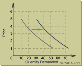
When there is a change in an influencing factor other than price, there may be a shift in the demand curve to the left or to the right, as the quantity demanded increases or decreases at a given price. For example, if there is a positive news report about the product, the quantity demanded at each price may increase, as demonstrated by the demand curve shifting to the right:

Demand Curve Shift
A number of factors may influence the demand for a product, and changes in one or more of those factors may cause a shift in the demand curve. Some of these demand-shifting factors are:

* Customer preference
*Prices of related goods
o Complements - an increase in the price of a complement reduces demand, shifting the demand curve to the left.
o Substitutes - an increase in the price of a substitute product increases demand, shifting the demand curve to the right.
*Income - an increase in income shifts the demand curve of normal goods to the right.
*Number of potential buyers - an increase in population or market size shifts the demand curve to the right.
*Expectations of a price change - a news report predicting higher prices in the future can increase the current demand as customers increase the quantity they purchase in anticipation of the price change.

Source: www.netmba.com

MBA Finance Topics-FINANCIAL RATIOS

Financial ratios are useful indicators of a firm's performance and financial situation. Most ratios can be calculated from information provided by the financial statements. Financial ratios can be used to analyze trends and to compare the firm's financials to those of other firms. In some cases, ratio analysis can predict future bankruptcy.

Financial ratios can be classified according to the information they provide. The following types of ratios frequently are used:

* Liquidity ratios
* Asset turnover ratios
* Financial leverage ratios
* Profitability ratios
* Dividend policy ratios

Liquidity Ratios

Liquidity ratios provide information about a firm's ability to meet its short-term financial obligations. They are of particular interest to those extending short-term credit to the firm. Two frequently-used liquidity ratios are the current ratio (or working capital ratio) and the quick ratio.

The current ratio is the ratio of current assets to current liabilities:

=	Current Assets Current Liabilities

Short-term creditors prefer a high current ratio since it reduces their risk. Shareholders may prefer a lower current ratio so that more of the firm's assets are working to grow the business. Typical values for the current ratio vary by firm and industry. For example, firms in cyclical industries may maintain a higher current ratio in order to remain solvent during downturns.
One drawback of the current ratio is that inventory may include many items that are difficult to liquidate quickly and that have uncertain liquidation values. The quick ratio is an alternative measure of liquidity that does not include inventory in the current assets. The quick ratio is defined as follows:

Quick Ratio

=

Current Assets - Inventory Current Liabilities

The current assets used in the quick ratio are cash, accounts receivable, and notes receivable. These assets essentially are current assets less inventory. The quick ratio often is referred to as the acid test.
Finally, the cash ratio is the most conservative liquidity ratio. It excludes all current assets except the most liquid: cash and cash equivalents. The cash ratio is defined as follows:

Cash Ratio

=

Cash + Marketable Securities Current Liabilities

The cash ratio is an indication of the firm's ability to pay off its current liabilities if for some reason immediate payment were demanded.

Asset Turnover Ratios

Asset turnover ratios indicate of how efficiently the firm utilizes its assets. They sometimes are referred to as efficiency ratios, asset utilization ratios, or asset management ratios. Two commonly used asset turnover ratios are receivables turnover and inventory turnover.
Receivables turnover is an indication of how quickly the firm collects its accounts receivables and is defined as follows:

Receivables Turnover

=

Annual Credit Sales Accounts Receivable

The receivables turnover often is reported in terms of the number of days that credit sales remain in accounts receivable before they are collected. This number is known as the collection period. It is the accounts receivable balance divided by the average daily credit sales, calculated as follows:

Average Collection Period

=

Accounts Receivable Annual Credit Sales / 365

The collection period also can be written as:

Average Collection Period

=

365 Receivables Turnover

Another major asset turnover ratio is inventory turnover. It is the cost of goods sold in a time period divided by the average inventory level during that period:

Inventory Turnover

=

Cost of Goods Sold Average Inventory

The inventory turnover often is reported as the inventory period, which is the number of days worth of inventory on hand, calculated by dividing the inventory by the average daily cost of goods sold:

Inventory Period

=

Average Inventory Annual Cost of Goods Sold / 365

The inventory period also can be written as:

Inventory Period

=

365 Inventory Turnover

Other asset turnover ratios include fixed asset turnover and total asset turnover.

Financial Leverage Ratios

Financial leverage ratios provide an indication of the long-term solvency of the firm. Unlike liquidity ratios that are concerned with short-term assets and liabilities, financial leverage ratios measure the extent to which the firm is using long term debt.
The debt ratio is defined as total debt divided by total assets:

Debt Ratio

=

Total Debt Total Assets

The debt-to-equity ratio is total debt divided by total equity:

Debt-to-Equity Ratio

=

Total Debt Total Equity

Debt ratios depend on the classification of long-term leases and on the classification of some items as long-term debt or equity.
The times interest earned ratio indicates how well the firm's earnings can cover the interest payments on its debt. This ratio also is known as the interest coverage and is calculated as follows:

Interest Coverage

=

EBIT Interest Charges

where EBIT = Earnings Before Interest and Taxes

Profitability Ratios

Profitability ratios offer several different measures of the success of the firm at generating profits.
The gross profit margin is a measure of the gross profit earned on sales. The gross profit margin considers the firm's cost of goods sold, but does not include other costs. It is defined as follows:

Gross Profit Margin

=

Sales - Cost of Goods Sold Sales

Return on assets is a measure of how effectively the firm's assets are being used to generate profits. It is defined as:

Return on Assets

=

Net Income Total Assets

Return on equity is the bottom line measure for the shareholders, measuring the profits earned for each dollar invested in the firm's stock. Return on equity is defined as follows:

Return on Equity

=

Net Income Shareholder Equity

Dividend Policy Ratios

Dividend policy ratios provide insight into the dividend policy of the firm and the prospects for future growth. Two commonly used ratios are the dividend yield and payout ratio.
The dividend yield is defined as follows:

Dividend Yield

=

Dividends Per Share Share Price

A high dividend yield does not necessarily translate into a high future rate of return. It is important to consider the prospects for continuing and increasing the dividend in the future. The dividend payout ratio is helpful in this regard, and is defined as follows:

Payout Ratio

=

Dividends Per Share Earnings Per Share

Use and Limitations of Financial Ratios

Attention should be given to the following issues when using financial ratios:

• A reference point is needed. To to be meaningful, most ratios must be compared to historical values of the same firm, the firm's forecasts, or ratios of similar firms.
• Most ratios by themselves are not highly meaningful. They should be viewed as indicators, with several of them combined to paint a picture of the firm's situation.
• Year-end values may not be representative. Certain account balances that are used to calculate ratios may increase or decrease at the end of the accounting period because of seasonal factors. Such changes may distort the value of the ratio. Average values should be used when they are available.
• Ratios are subject to the limitations of accounting methods. Different accounting choices may result in significantly different ratio values.
  
  Source: www.netmba.com

MBA Finance Topics-Common Size Financial Statements

Common size ratios are used to compare financial statements of different-size companies, or of the same company over different periods. By expressing the items in proportion to some size-related measure, standardized financial statements can be created, revealing trends and providing insight into how the different companies compare.

The common size ratio for each line on the financial statement is calculated as follows:

Common Size Ratio

=

Item of Interest Reference Item

For example, if the item of interest is inventory and it is referenced to total assets (as it normally would be), the common size ratio would be:

Common Size Ratio for Inventory

=

Inventory Total Assets

The ratios often are expressed as percentages of the reference amount. Common size statements usually are prepared for the income statement and balance sheet, expressing information as follows:

• Income statement items - expressed as a percentage of total revenue
• Balance sheet items - expressed as a percentage of total assets

The following example income statement shows both the dollar amounts and the common size ratios:

Common Size Income Statement

	Income Statement	Common-Size Income Statement
Revenue	70,134	100%
Cost of Goods Sold	44,221	63.1%
Gross Profit	25,913	36.9%
SG&A Expense	13,531	19.3%
Operating Income	12,382	17.7%
Interest Expense	2,862	4.1%
Provision for Taxes	3,766	5.4%
Net Income	5,754	8.2%

For the balance sheet, the common size percentages are referenced to the total assets. The following sample balance sheet shows both the dollar amounts and the common size ratios:

Common Size Balance Sheet

	Balance Sheet	Common-Size Balance Sheet
ASSETS
Cash & Marketable Securities	6,029	15.1%
Accounts Receivable	14,378	36.0%
Inventory	17,136	42.9%
Total Current Assets	37,543	93.9%
Property, Plant, & Equipment	2,442	6.1%
Total Assets	39,985	100%
LIABILITIES AND SHAREHOLDERS' EQUITY
Current Liabilities	14,251	35.6%
Long-Term Debt	12,624	31.6%
Total Liabilities	26,875	67.2%
Shareholders' Equity	13,110	32.8%
Total Liabilities & Equity	39,985	100%

The above common size statements are prepared in a vertical analysis, referencing each line on the financial statement to a total value on the statement in a given period.
The ratios in common size statements tend to have less variation than the absolute values themselves, and trends in the ratios can reveal important changes in the business. Historical comparisons can be made in a time-series analysis to identify such trends.
Common size statements also can be used to compare the firm to other firms.

Comparisons Between Companies (Cross-Sectional Analysis)

Common size financial statements can be used to compare multiple companies at the same point in time. A common-size analysis is especially useful when comparing companies of different sizes. It often is insightful to compare a firm to the best performing firm in its industry (benchmarking). A firm also can be compared to its industry as a whole. To compare to the industry, the ratios are calculated for each firm in the industry and an average for the industry is calculated. Comparative statements then may be constructed with the company of interest in one column and the industry averages in another. The result is a quick overview of where the firm stands in the industry with respect to key items on the financial statements.

Limitations

As with financial statements in general, the interpretation of common size statements is subject to many of the limitations in the accounting data used to construct them. For example:

• Different accounting policies may be used by different firms or within the same firm at different points in time. Adjustments should be made for such differences.
• Different firms may use different accounting calendars, so the accounting periods may not be directly comparable.

Source: www.netmba.com

MBA Finance Topics-CAPITAL BUDGETING

A capital expenditure is an outlay of cash for a project that is expected to produce a cash inflow over a period of time exceeding one year. Examples of projects include investments in property, plant, and equipment, research and development projects, large advertising campaigns, or any other project that requires a capital expenditure and generates a future cash flow.

Because capital expenditures can be very large and have a significant impact on the financial performance of the firm, great importance is placed on project selection. This process is called capital budgeting.

Criteria for Capital Budgeting Decisions

Potentially, there is a wide array of criteria for selecting projects. Some shareholders may want the firm to select projects that will show immediate surges in cash inflow, others may want to emphasize long-term growth with little importance on short-term performance. Viewed in this way, it would be quite difficult to satisfy the differing interests of all the shareholders. Fortunately, there is a solution.

The goal of the firm is to maximize present shareholder value. This goal implies that projects should be undertaken that result in a positive net present value, that is, the present value of the expected cash inflow less the present value of the required capital expenditures. Using net present value (NPV) as a measure, capital budgeting involves selecting those projects that increase the value of the firm because they have a positive NPV. The timing and growth rate of the incoming cash flow is important only to the extent of its impact on NPV.

Using NPV as the criterion by which to select projects assumes efficient capital markets so that the firm has access to whatever capital is needed to pursue the positive NPV projects. In situations where this is not the case, there may be capital rationing and the capital budgeting process becomes more complex.

Note that it is not the responsibility of the firm to decide whether to please particular groups of shareholders who prefer longer or shorter term results. Once the firm has selected the projects to maximize its net present value, it is up to the individual shareholders to use the capital markets to borrow or lend in order to move the exact timing of their own cash inflows forward or backward. This idea is crucial in the principal-agent relationship that exists between shareholders and corporate managers. Even though each may have their own individual preferences, the common goal is that of maximizing the present value of the corporation.
Alternative Rules for Capital Budgeting

While net present value is the rule that always maximizes shareholder value, some firms use other criteria for their capital budgeting decisions, such as:

* Internal Rate of Return (IRR)
* Profitability Index
* Payback Period
* Return on Book Value

In some cases, the investment decisions resulting from the IRR and profitability index methods agree with those of NPV. Decisions made using the payback period and return on book value methods usually are suboptimal from the standpoint of maximizing shareholder value.

Source: www.netmba.com

MBA Finance Topics-PERPETUITIES

A perpetuity is a series of equal payments over an infinite time period into the future. Consider the case of a cash payment C made at the end of each year at interest rate i, as shown in the following time line:

Perpetuity Time Line

0		1		2		3
PV		C		C		C

Because this cash flow continues forever, the present value is given by an infinite series:

PV = C / ( 1 + i ) + C / ( 1 + i )² + C / ( 1 + i )³ + . . .

From this infinite series, a usable present value formula can be derived by first dividing each side by ( 1 + i ).

PV / ( 1 + i ) = C / ( 1 + i )² + C / ( 1 + i )³ + C / ( 1 + i )⁴ + . . .

In order to eliminate most of the terms in the series, subtract the second equation from the first equation:

PV - PV / ( 1 + i ) = C / ( 1 + i )

Solving for PV, the present value of a perpetuity is given by:

PV =

C i

Growing Perpetuities

Sometimes the payments in a perpetuity are not constant but rather, increase at a certain growth rate g as depicted in the following time line:

Growing Perpetuity Time Line

0		1		2		3
PV		C		C(1+g)		C(1+g)2

The present value of a growing perpetuity can be written as the following infinite series:

PV =

C ( 1 + i )

+

C ( 1 + g ) ( 1 + i )2

+

C ( 1 + g )2 ( 1 + i )3

+ . . .

To simplify this expression, first multiply each side by (1 + g) / (1 + i):

PV ( 1 + g) ( 1 + i )

=

C ( 1 + g ) ( 1 + i )2

+

C ( 1 + g )2 ( 1 + i )3

+ . . .

Then subtract the second equation from the first:

PV -

PV ( 1 + g) ( 1 + i )

=

C ( 1 + i )

Finally, solving for PV yields the expression for the present value of a growing perpetuity:

PV =

C i - g

For this expression to be valid, the growth rate must be less than the interest rate, that is, g < i .

Source: www.netmba.com